Attention Based Masking for Vision Transformer Pretraining

Evaluating Guided Masking Strategies for MultiMAE

Research ProjectComputer VisionDLCV 2022/2023

Overview

The Problem

MultiMAE extends Masked Autoencoders to multiple modalities (RGB, depth, semantic segmentation) by randomly masking approximatelycode.math-inline $83\%$ of input tokens. However, not all patches carry the same information. Patches covering the actual subject are far more informative than background patches. Random masking may not create the most effective pretext task for learning rich representations.

The Solution

We replace random patch sampling with attention-guided masking: a quick forward pass produces per-token attention scores, and we mask the highest-attention patches before the actual training step:

\mathcal{M} = \text{top-}k(\{A_i\})

This forces the model to reconstruct what it cares about most: a harder, more useful pretext task. Continuing pretraining for only 100 additional epochs on top of the public 1600-epoch MultiMAE checkpoint, this outperforms the random-masking baseline on ImageNet-1K classification and NYUv2 segmentation.

Background

Masked Autoencoders (MAE)

MAEs learn visual representations by reconstructing randomly masked image patches. The image is split intocode.math-inline $N$ patches, approximatelycode.math-inline $75%$ are hidden, and a transformer encoder-decoder reconstructs them. The encoder is kept for downstream tasks.

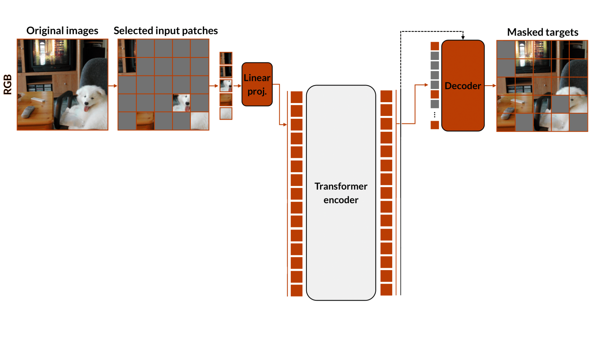
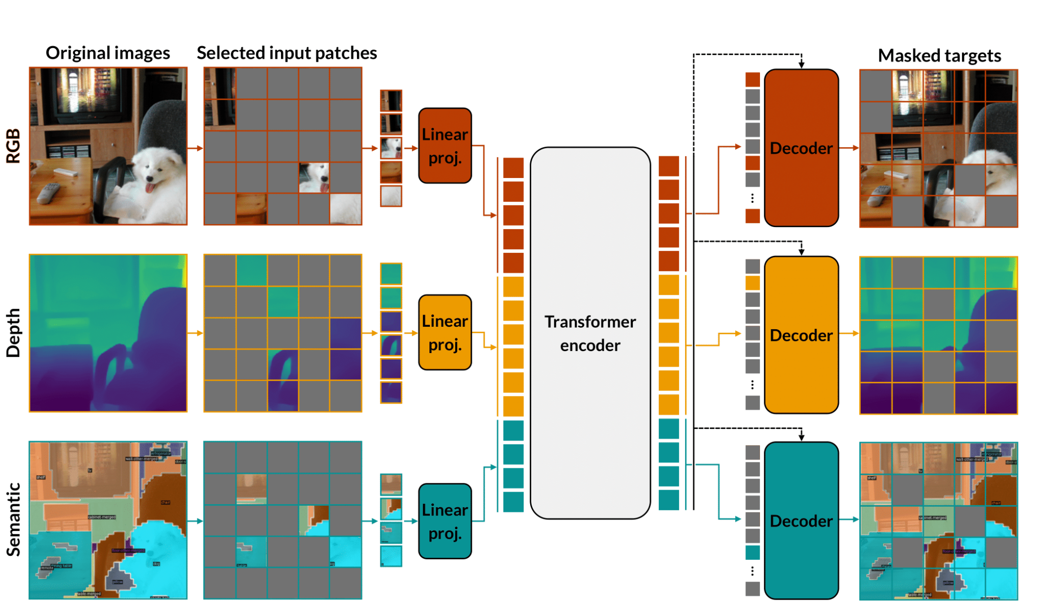
MultiMAE

MultiMAE extends MAE to multiple modalities (RGB, depth, and semantic segmentation) jointly tokenized and encoded by a shared transformer with per-modality decoders. Approximatelycode.math-inline $83%$ of input tokens are dropped before the encoder.

Informed Masking (AttMask)

AttMask showed that for DINO, masking is more useful when it is informed: hiding the patches the model attends to most produces a harder, more useful pretext task.

Method: Attention-Guided Masking

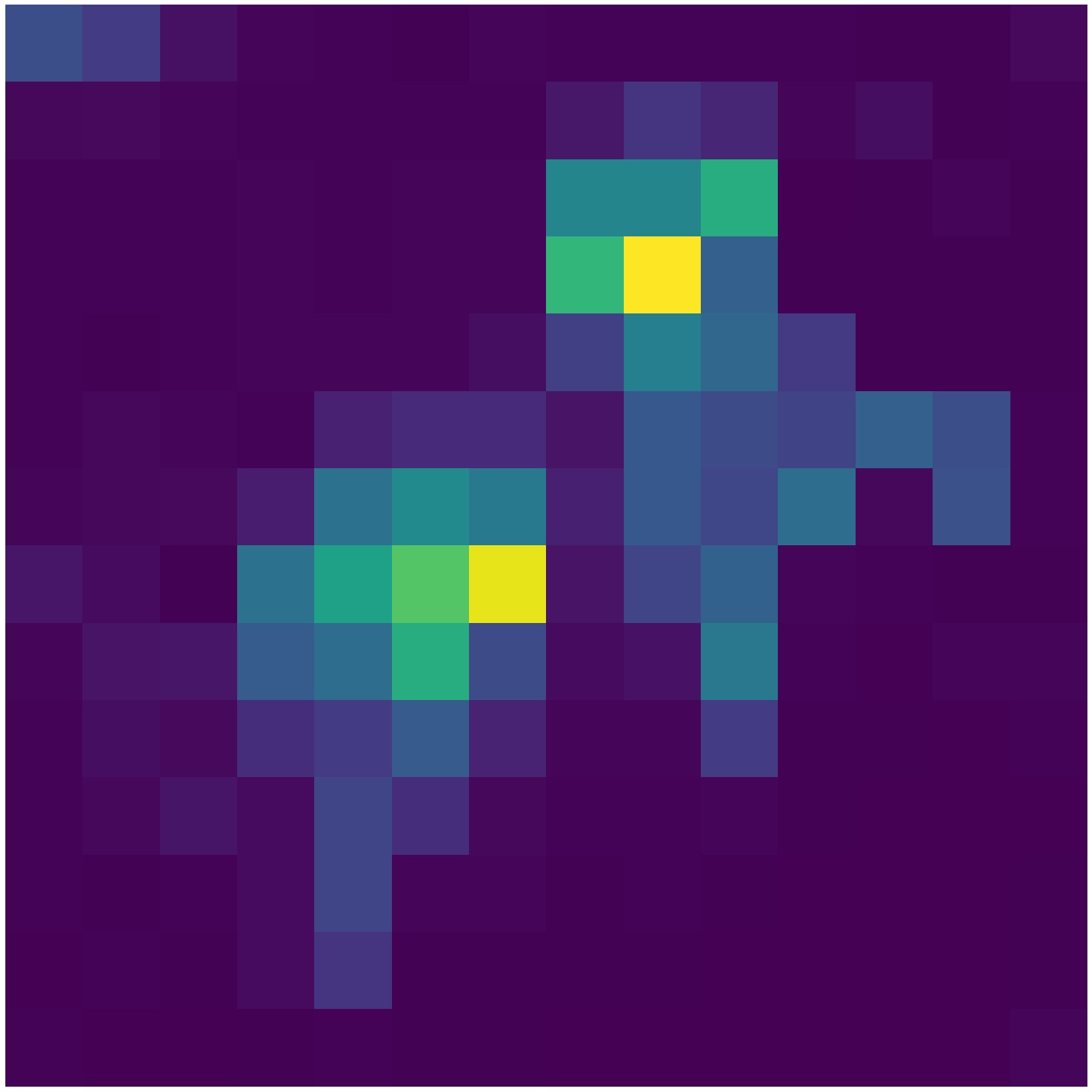
Computing per-token attention

Before the actual training step, we run one extra encoder forward pass without masking over all tokens of all modalities. From the last transformer layer we read out the attention weightscode.math-inline $A_{ij}$ average across allcode.math-inline $H$ heads, and obtain a single attention score per token:

\bar{A}_i = \frac{1}{H} \sum_{h=1}^{H} A_i^{(h)}

Attention computation across modalities in MultiMAE

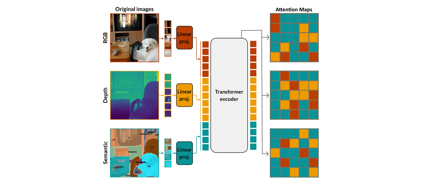
Masking with the attention map

The number of tokens drawn from each modality is sampled from a symmetric Dirichlet distributioncode.math-inline $\text{Dir}(\alpha, \alpha, \alpha)$ , and within each modality we mask the patches with the highest attention, keeping the same overall masking ratio of approximately 83%.

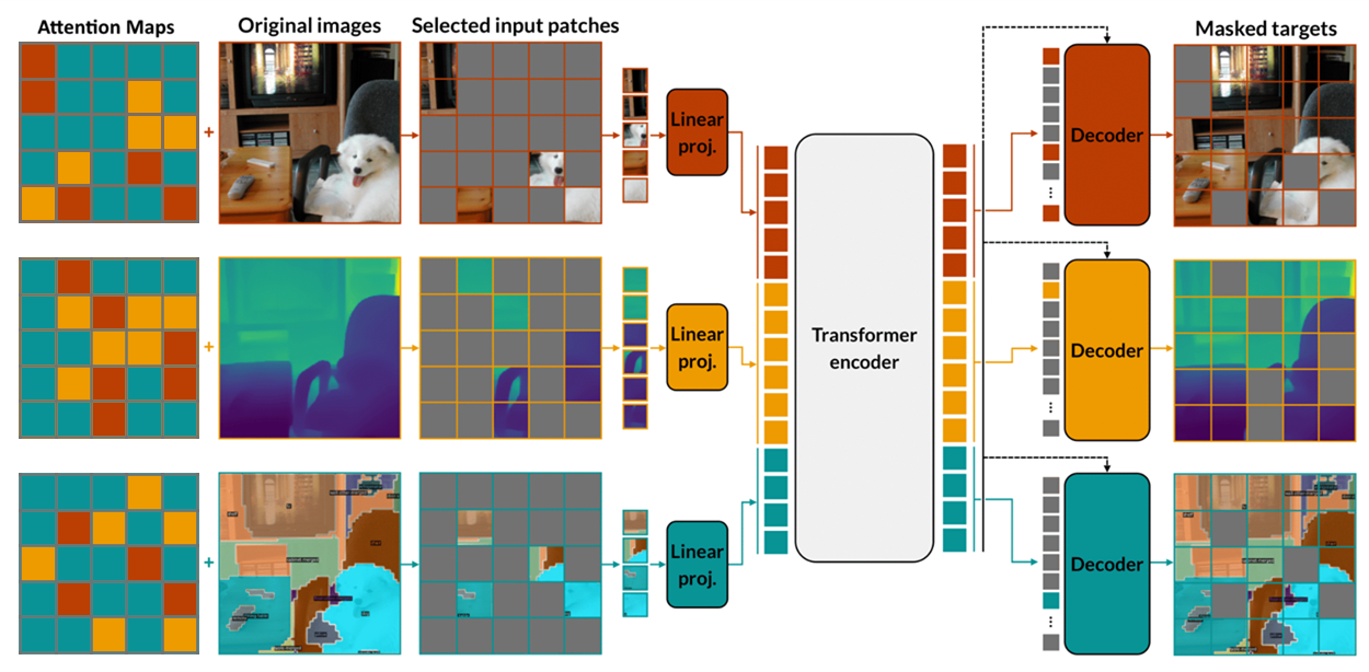
Full attention-masking pipeline with cached embeddings

The token embeddings produced by the linear projection during the attention pass are cached and reused for the actual encoder pass, so the only added cost is one extra encoder forward, not a second full pretraining stage.

Setup

A full MultiMAE pretraining run takes approximately 96 days on 2x A6000 GPUs. Rather than retrain from scratch, we continue pretraining from the public 1600-epoch checkpoint for 100 additional epochs (approximately 6 days) with our attention-guided masking, then finetune on each downstream task. Practically this means our run lives on the very lastcode.math-inline $\approx 1/16$ th of the original cosine learning rate schedule:

\eta_t = \eta_{\min} + \frac{1}{2}(\eta_{\max} - \eta_{\min})(1 + \cos(\frac{t}{T_{\max}}\pi))

where the learning rate is already small at the end of training.

Baseline Results

Despite only 100 epochs of continued pretraining, attention-guided masking matches or slightly outperforms random masking across all three benchmarks:

Task	Baseline (paper)	Baseline (reproduced)	Attention (ours)
Classification / IN1K [Acc]	83.3	83.3	83.5
SemSeg / ADE20K [mIoU]	46.2	47.0	46.9
SemSeg / NYUv2 [mIoU]	52.0	51.5	51.6

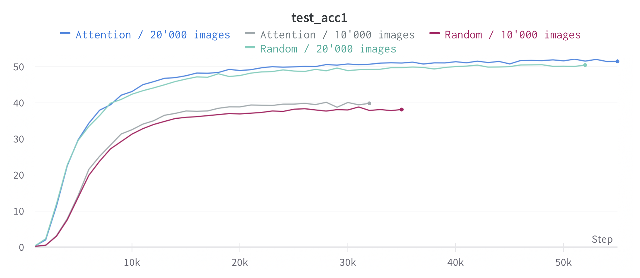
When we restrict the IN1K finetuning data to small subsets, the gap to random masking widens: a small but encouraging signal that attention-based pretraining generalizes better in the low-data regime:

IN1K finetuning accuracy on 10k / 20k image subsets

Variants and Ablations

5.1 Higher Learning Rate

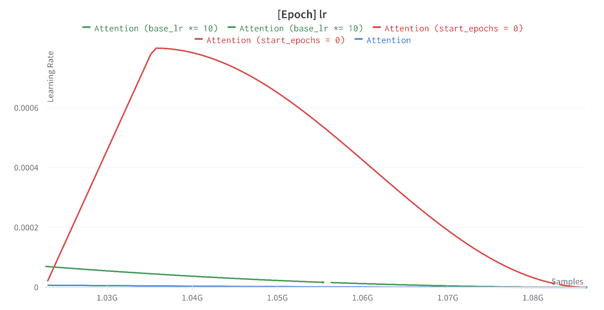
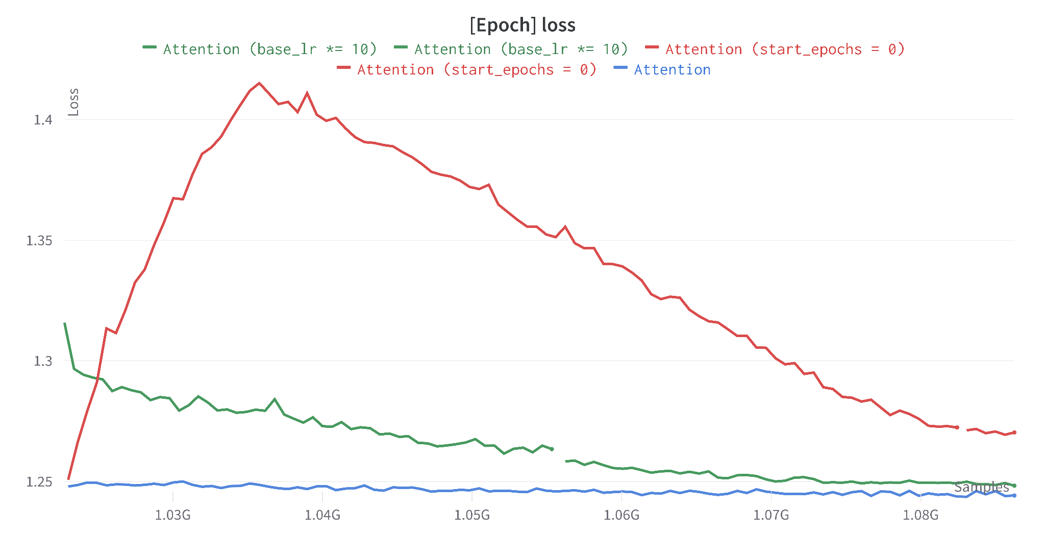
Because we only ride the tail of the original cosine schedule, the effective learning rate during our 100-epoch continuation is tiny. We tested two countermeasures:

start_epochs = 0: restart the cosine schedule from scratch over the 100 continuation epochs (with a 20-epoch warmup).
base_lr × 10: keep the schedule but multiply the base learning rate by 10.

LR curves for the three runs: original tail, ×10 base LR, full restart

Pretraining loss for the three LR variants

	Baseline	Attention	Attention start_epochs=0	Attention base_lr×10
IN1K [Acc]	83.3	83.5	83.3	83.4
ADE20K [mIoU]	47.0	46.9	46.6	46.3
NYUv2 [mIoU]	51.5	51.6	–	–

Takeaway: A higher LR likely needs many more epochs to re-converge. With our 100-epoch budget, the conservative tail of the original schedule is the right call.

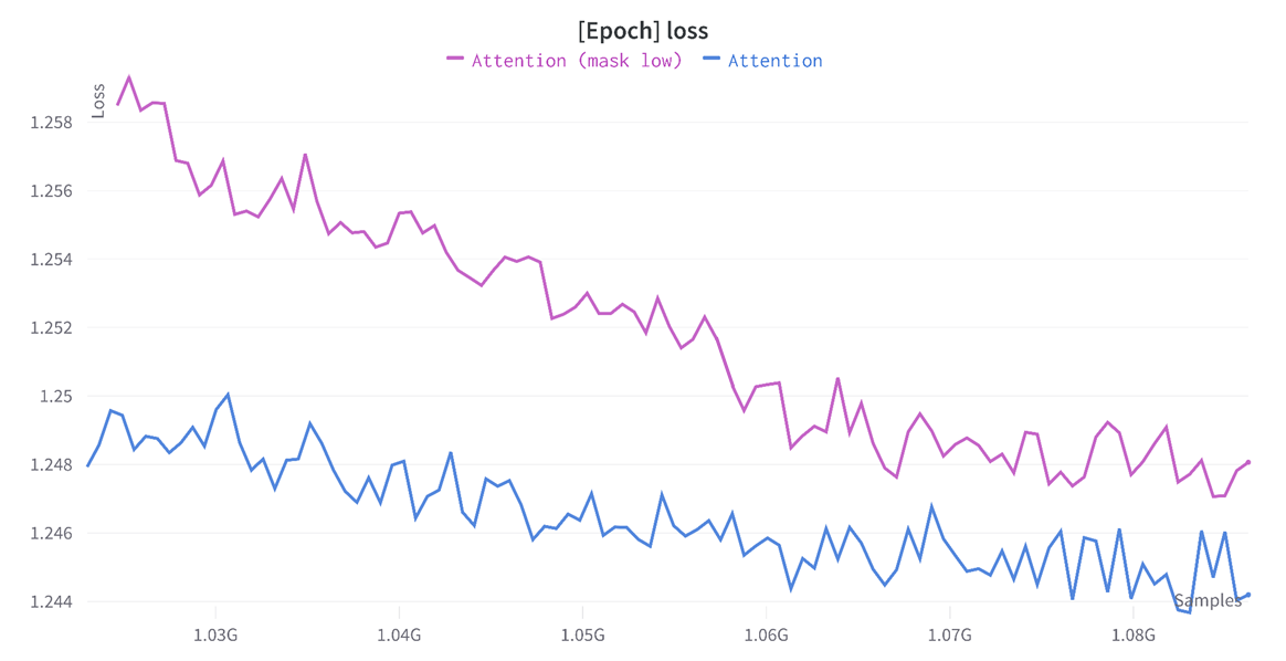
5.2 Inverse Masking

Default attention masking hides high-attention patches, forcing the model to reconstruct what it cares about. The inverse strategy hides low-attention patches and lets the encoder concentrate on the relevant region:

\mathcal{M}_{\text{high}} = \{i \mid A_i \in \text{top-}k(\{A_j\})\}

\mathcal{M}_{\text{low}} = \{i \mid A_i \in \text{bottom-}k(\{A_j\})\}

Pretraining loss: mask-low vs. mask-high

	Baseline	Attention (high masking)	Attention (low masking)
IN1K [Acc]	83.3	83.5	83.3
ADE20K [mIoU]	47.0	46.9	46.78
NYUv2 [mIoU]	51.5	51.6	51.63

Takeaway: To learn a better representation, the model has to be denied the most informative patches, confirming the AttMask intuition in the multi-modal setting.

5.3 Stochastic Attention Masking

Pure top-k selection from the attention map can be too rigid. We add controlled Gaussian noise to the attention scores before selecting which patches to mask:

\tilde{A} = \alpha \cdot \mathcal{N}(\mu(A), \sigma(A)) + (1 - \alpha) \cdot A

where α in [0, 1] controls the stochasticity, and the noise is calibrated to the per-image attention statistics.

	Baseline	Attention
IN1K [Acc]	83.3	83.5
ADE20K [mIoU]	47.0	46.9
NYUv2 [mIoU]	51.5	51.6

5.4 Random Attention-Head Ensemble

Averaging attention across all heads can wash out useful per-head signal. We tried sampling a random subset of headscode.math-inline $h \sim \text{Uniform}(1, H)$ each step instead:

\bar{A}_i^{\text{sparse}} = \frac{1}{|\mathcal{H}|} \sum_{h \in \mathcal{H}} A_i^{(h)}, \quad \mathcal{H} \subset \{1,\ldots,H\}

This produced a higher evaluation loss when used for masking, suggesting the averaged attention map was already the more reliable signal.

Summary of Results

	Baseline	Attention mask_high	Attention mask_low	Attention lr×10	Attention e=0
IN1K [Acc]	83.3	83.5	83.3	83.4	83.3
ADE20K [mIoU]	47.0	46.9	46.78	46.3	46.6
NYUv2 [mIoU]	51.5	51.6	51.63	51.32	50.27

Conclusions

Key Findings

Vanilla attention masking: even with only 100 continuation epochs, outperforms a random-masking baseline on IN1K and NYUv2, and matches it on ADE20K.
Attention-guided masking is not robust to LR changes: increasing the LR consistently hurt downstream performance under our 100-epoch budget.
Inverse masking confirms the core intuition: to learn a better representation the model has to be denied the most informative patches.
The strongest variant remains the simplest: cache embeddings from a no-mask forward pass, mask the top-attention tokens, train as usual.

Future Work

Uncertainty-guided masking: use per-patch reconstruction loss as uncertainty signal: $U_i = \mathcal{L}_{\text{recon}}(x_i, \hat{x}_i)$ (too compute-heavy for this project).
Tokens-per-modality Dirichlet sampling: bias sampler toward harder modalities using asymmetric Dirichlet distribution: $\boldsymbol{\pi} \sim \text{Dir}(\alpha_1, \alpha_2, \alpha_3)$ wherecode.math-inline $\alpha_m$ is driven by moving averages of per-modality losses.
400-epoch from-scratch run: with attention masking - compute, not method, was the binding constraint.

Project Info

Course: DLCV 2022/2023 Final Project
Affiliation: Technische Universität Darmstadt, Visual Inference Lab
Code: Built on top of EPFL-VILAB/MultiMAE

For inquiries about collaboration or research opportunities

Contact Leon Camus